|
Analysis of the Economic Impact of the US-Australia Free Trade Agreement ―Focusing on Agricultural Issues― |
|
2. Analysis of Trade Liberalization Negotiations, Based on Bargaining Theory 3. US-Australia Free Trade Agreement 4. Economic Impact of the US-Australia Free Trade Agreement |
|||
|
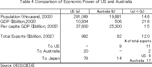
4.Economic Impact of the US-Australia Free Trade Agreement (1) Outline of the Economic Power of Both Countries Firstly, population, GDP, trade amount and other basic data are briefly presented in Table 4 for comparing the economic power of the US and Australia. The US has a total population of 290 million, 14.6 times as many as Australia's 20 million. The US GDP is $11 trillion, 21.6 times Australia's $500 billion. The US per capita GDP amounts to $37,600, 1.5 times Australia's $25,300. Seeing the major economic indices as above, the scale of the US economy is huge, 15 to 20 times that of Australia.
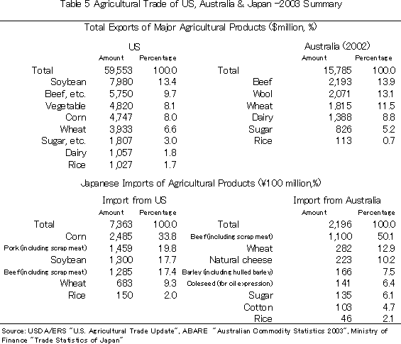
US exports amount to $982 billion, 12 times Australia' s $82 billion. Trade between the US and Australia is also asymmetrical. US exports to Australia amount to $20 billion, accounting for 2% of its total exports. Australia's exports to the US total $9 billion, accounting for 11% of the total. The US is the 3rd largest importer of Australian goods, after Japan (17% of total Australia's exports) and the EU (14%). But it should be said that Australia, as a trade partner, carries far less weight than the US. Further looking into the exports of agricultural goods from both countries (Table 5), US exports amounted to about $60 billion in 2003. The major agricultural products exported by the US are soybeans, valued at $7,980 million (13.4% of total export of agricultural products), beef, etc. valued $5,750 million (9.7% of the total), vegetables at $4,820 million (8.1%), corn at $4,747 million (8.0%) and so on. Meanwhile, Australia's exports of agricultural products amounted to about $16 billion in 2002. The major export agricultural products were beef, valued at $2,193 million (13.9% of total agricultural export), wool and wool products at $2,071 million (13.1%),wheat $1,815 million (11.5%), dairy products $1,388 million (8.8%), sugar $826 million (5.2%), etc. Additionally, in 2003 Japan imported corn valued at
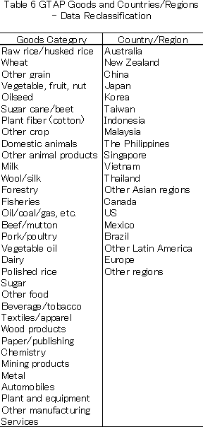
(2) GTAP and Past Researches GTAP is a tool for analyzing the impact of a change in tariff or export subsidy on production or trade from a global viewpoint within the framework of general equilibrium analysis. To name literature that details GTAP, Hertel's [6] will be a typical text for further details. In a general equilibrium model, economic agents such as households maximize utility under budgetary constraint or those such as enterprises maximize profit under the constraint of the production function in a perfectly competitive economy. GTAP makes it possible to compute and analyze what change is caused in the model-calculated equilibrium prices and quantities at the time of a policy change, for instance, tariff reduction, based on the actual data. A shock or change resultant from tariff reduction or elimination in the market of goods affects derived demand for the production factors needed in production. For example, if demand for wheat increases for a certain reason and wheat production is boosted, demands for primary factors of production such as labor, land and capital and intermediate goods increase, derived from wheat production. If the supply of primary factors is fixed, an increase in derived demand for primary factors in the wheat sector decreases derived demand in the other sector. This sort of change causes a change in income. As GTAP is a general equilibrium model, it can describe the changes in the overall economy in a unified way. And it is able to make a calculation in a form of equivalent variation by countries for judging whether a certain shock has a favorable impact or not, taking into consideration various influences comprehensively. GTAP used here is version 5. Version 5 has a somewhat old datum point in 1997. In this paper the equilibrium in 1997 and the equilibrium to be newly formed by the tariff deduction, which is presumed on a case-by-case basis, are comparatively analyzed. As already seen, some tariff rates will be reduced by stages. Also, it would take some time to make adjustment such as the shift between production factors until a new equilibrium forms after a shock. However, any such thing is disregarded and any change is deemed adjusted momentarily. This assumption that neglects any adjustment implies that the analysis aims at the middle-term effect of a change in tariff rate on the economy. Also, such impact or effect as an increase in investment, acceleration of competition or progress in technology is entirely disregarded, and only the simple static effect of tariff rate reduction is measured. Berkelmans, et al. [3] and the Centre for International Economics [4] measured the economic impact of the US-Australia FTA. The former analyzes the economic impact expected in each sector, using GTAP, before the US-Australia FTA negotiation, and it is needless to say that it offers no analysis on the compromise made this time. The latter analyzes the impact of the US-Australia FTA as concluded by the G-cubed model, a dynamic general equilibrium model, and indicated that the FTA would serve to push up Australia's real GDP by $6.1 billion (+0.7%). It also offers detailed sector-by-sector analysis on the effect of the Agreement, but it is not a comparative analysis to ascertain the economic losses of the compromise by comparing perfect tariff elimination and the agreed scheme, but only offers analysis on the sector-by-sector change in production or export/import, lacking study of the effect of the compromise. Furthermore, neither analysis pays attention to the economic impact of the US-Australia FTA on Japan. (3) Data and Scenario One strength of GTAP would be that it offers a "quite segmented analysis of agriculture for a general equilibrium model covering all industries". When segmentation is made to the limit, employing GTAP version 5, 57 categories of goods in 66 countries/regions can be analyzed. In this paper these regions and goods are re-grouped into 20 countries/regions and 33 categories of goods, and the results are calculated. Table 6 details such calculation. As the main purpose is to analyze the impact on the agricultural sector, the category of goods is made more detailed for agricultural and fishery products and simplified in other industries, with several industries summed up.
As already mentioned, the US-Australia FTA is not a free trade agreement, excluding sugar, dairy, etc. What a difference does this sort of exception make on economic impact, compared with perfect free trade? Now it is assumed as Case 1 that the US and Australia both eliminate any tariff on imports from the other country. On the other hand, if based on the draft agreement, it is necessary to recreate the tariff quota system of the US for sugar, dairy, etc. When a tariff quota system is directly expressed in GTAP, however, it is necessary to add new data concerning model adjustment or tariff quota system. Here the tariff quota system itself is not expressed directly, but the barrier for the excepted goods is converted into tariff rate equivalent. Specifically speaking, the tariff rate on sugar is not changed, but kept at the level of the datum point. The tariff quota is maintained for dairy products, so that the products are made subject to a 4.1% tariff rate of the US, based on CIE [4] estimation. It is scheduled that tariffs will be finally eliminated for beef, so the US tariff rate is set at zero. With respect to the other products, the tariff rate is assumed to be zero as in Case 1. These assumptions constitute Case 2 based on the draft agreement, and this is compared with Case 1. In addition, a BSE-infected cow was found in December 2003 and Japan and several other countries are temporarily suspending beef imports from US as of May 2005. Also, beef imports from Canada are temporarily suspended, as a BSE-infected cow was confirmed there in May 2003. However, the effect of these events is deemed tentative until safety is reconfirmed. Therefore, the effect is not considered in this analysis, and it is assumed that all countries are importing beef from US and Canada under normal conditions (1). (4) Result of Analysis 1) Equivalent Variation and GDP In Table 7 the equivalent variation of each country is shown for both cases. For Australia it increases slightly by $44.3 million in Case 1 of perfect tariff elimination but decreases by $42.6 million in Case 2, which is based on the draft agreement excepting some agricultural products. In order to conclude whether the US-Australia FTA as agreed has an adverse effect on Australia, a further examination or analysis considering dynamic effects, for instance, is necessary. However, it may be well imagined that the compromise, which has allowed the US to keep the tariff quota system on imported sugar and dairy, costs Australia at least $80 million, compared with perfect trade liberalization. Meanwhile, the US gains $378.9 million in Case 1 and $456.9 million in Case 2. The difference between Case 1 and Case 2 only amounts to $78 million, but the equivalent variation becomes larger in Case 2 than Case 1. Thus, it can be said that the agreement as drafted is more favorable for the US.
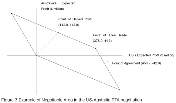
Any third party country other than the US and Australia has a minus equivalent variation regardless of Case 1 or 2. Japan's equivalent variation is minus $110.2 million in Case 1 and minus $98.8 million in Case 2, and Europe's minus $134.2 in Case 1 and minus 133.6 million in Case 2. The world total of equivalent variations for these countries and regions being the third parties amounts to minus $116.3 million in Case 1 and minus $49.7 million in Case 2. The US-Australia FTA itself, either in the case of perfect tariff elimination or as agreed, is not favorable from a worldwide viewpoint. But the negative impact of the compromise in the agreement as drafted is more than halved, compared with perfect free trade. The GDP changes by 0.02% in Australia, a party to the FTA, in Case 1 and minus 0.11% in Case 2. Even in Case 1 the GDP increase is very small and it turns negative in Case 2. The US GDP hardly changes either in Case 1 or 2; 0.03% in Case 1 and 0.04% in Case 2. For third party countries the impact is negative in either case. For Japan GDP hardly changes at minus 0.02% either in Case 1 or 2 and the change is minus 0.02% in Europe in either case. New Zealand suffers from a decrease in GDP of 0.12% in Case 1 and 0.13% in Case 2. As the country is strongly tied with Australia, it suffers from comparatively stronger impact as a third party. It is considered that New Zealand's agricultural exports to US will be driven out by Australia. Generally it could be said that the US-Australia FTA has a very small static effect on the overall economy in either country. The reason is that from the very start most of the high tariff goods are agricultural products, accounting for a small share of the overall economy, and the reduction in tariff rate therefore does not have much impact on the overall economy. Although the FTA has negative impacts on the overall economy of each third party country/region, including Japan and Europe, it has turned out to be less than free trade, and it could be said that the impact is very minor. 2) Application of Bargaining Theory In Section 2, the concept of probability has been introduced in the definitive analysis of a non-cooperative game and a solution of negotiation was analyzed. Now let us analyze the US-Australia FTA negotiation employing bargaining theory, assuming that equivalent variation is the profit gained by negotiation. First the point of reference, being the starting point of negotiation, is set to be the situation before negotiation begins, and equivalent variation is set at zero in both countries. Profit obtained in case of perfect tariff elimination by both countries has the equivalent variation gained in Case 1 set as the point of free trade. Finally profit obtained when one country keeps tariffs and the other country eliminates them is regarded as the equivalent variation respectively in case that the US (or Australia) keeps all tariff rates and Australia (or the US) sets all tariff rates at zero. Based on the above assumptions, Figure 3 charts the US-Australia FTA negotiation within the framework of the analysis by Riezman [8]. The horizontal axis represents a scale to measure the US's expected profit (equivalent variation) and the vertical axis shows Australia's. When one country keeps tariffs and the other eliminates them, the former party's equivalent variation=expected profit is positive but the latter party's becomes negative to a large extent. The point of free trade is the combination of equivalent variations of the US and Australia in Case 1. Looking individually, profit from free trade is bigger for the US and smaller for Australia. If negotiation addresses the maximization of the product of the profits obtained by both countries, the solution of negotiation is given when the profits both countries obtain are equal. In dollar terms, such obtained profit amounts to $142.0 million for each country. Meanwhile, profits calculated for the actually agreed scheme is the "point of agreement" in the same chart, far distant from a theoretical solution of negotiation and even out of the set of realizable negotiation away from the region of negotiation.
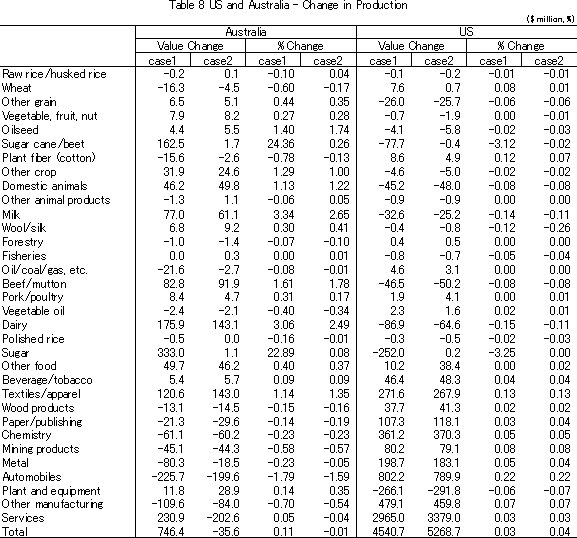
This set of realizable negotiation is charted by giving probability to definitive profit, not by manipulating the tariff rates of the US and Australia within GTAP. Accordingly all of the combinations of profit obtained by manipulating tariff rates on all products are not included in this set of realizable negotiation. In the first place the profit obtainable from negotiation must be larger than the point of reference. Otherwise, individual rationality is not met and negotiation becomes meaningless. However, Australia's profit calculated at the point of agreement is lower than Australia's point of reference, and is not included in the region for negotiation. The calculation results did not present any justifiable explanation on the ground of bargaining theory for Australia's acceptance of the agreement as drafted. However, the following two points are still open to dispute. In the first place only the static effect of the tariff elimination of the US-Australia FTA is handled in the model, and the results are not based on a comprehensive analysis including the dynamic effect of the liberalization of investment. Secondly the point of reference is placed time-wise before negotiation, but there is a possibility that a failure of negotiation may result in a level of welfare below the original level or otherwise the point of reference might shift to another position. Depending upon where the point of reference for negotiation is set, it would be possible to explain the formation of individual rationality of the agreement as drafted. For explaining why the US consistently maintained an obstinate stance and made a compromise in the field of agriculture it should also be pointed out that the economic effect of the US-Australia FTA is small and that exports to Australia hardly weigh for the US. The US-Australia FTA is estimated to generate potential economic advantage of $1.3 per head in the terms of equivalent variation in Case 1 for the US, well below Australia's $2.2. 3) Impact on Production (i) Production Value Table 8 sets forth the changes in production value both in the US and Australia. With Australia sugar production increases greatly by $333.0 million (+22.9%) in Case 1. And the production of sugar cane and sugar beet as material is expected to rise by $162.5 million (+24.4%). However, in Case 2 where sugar is treated as an exception, maintaining the status quo, its production only increases by $1.1 million (+0.08%). The production of sugar cane and sugar beet also increases slightly by $1.7 million (+0.26%). Not much change is made from the days before the FTA was concluded.
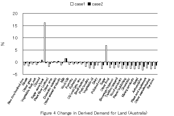
Next, dairy production increases by $175.9 million (+3.1%) in Case 1 and $143.1 million (+2.5%) in Case 2, where the increase is somewhat lower in percentage but substantial in amount. And the production of milk, the material for dairy products, increases by $77.0 million (+3.3%) in Case 1 and $61.1 million (+2.7%) in Case 2. As for dairy the US maintains its tariff quota system, but is planning to establish and broaden the quota. Therefore, the impact is very different from sugar on which TRQ is maintained as it is. With respect to beef it is expected that the tariff quota system is maintained for 20 years or so, and the barrier will be gradually eliminated over a transition period. As the tariff quota system will be all eliminated finally, in this paper it is assumed that tariffs are completely eliminated on beef and beef products in Case 2 as well. Tariff elimination increases the production of beef, mutton and related products by $82.8 million (+1.6%) in Case 1 and by $91.9 million (+1.8%) in Case 2, more than Case 1. This is interpreted as an increase in production of beef, etc. to make up for the dull production increase of sugar and dairy. The production of livestock being intermediate goods is expected to increase by $46.2 million (+1.1%) and $49.8 million (+1.2%) in Case 2. There are some other agricultural products, whose production increase rate is higher in Case 2 than Case 1. Raw and husked rice, vegetables, fruits and nuts, oil seeds, wool and silk, etc. are such products. Also, some farm products decrease in production in both cases. Wheat production decreases by $16.3 million (-0.6%) in Case 1 and by $4.5 million (-0.2%) in Case 2. The decrease rate is smaller in Case 2, but production decreases in either case. Finally other food products are mentioned. The production also increases by $49.7 million (+0.4%) in Case 1 and by $46.2 million (+0.4%) in Case 2. Other than agricultural products, car production decreases by $199.6 million (-1.6%) in Case 2 and production decreases for most other products except clothes. Australia's overall production increases by $746.4 million (+0.1%) in Case 1 but slightly decreases by $35.6 million (-0.01%) in Case 2. On the part of the US, meanwhile, sugar production sharply decreases by $252.0 million (-3.3%) in Case 1 but increases slightly by $0.2 million (0.00%) in Case 2. For sugar cane and beet a production decrease is quite large in Case 1 but limited in Case 2. Dairy production decreases by $86.9 million (-0.15%) in Case 1 and less by $64.6 million (-0.11%) in Case 2. Milk production decreases as much as dairy. The production of beef and mutton also decreases but the drop is far smaller by $46.5 million (-0.08%) in Case 1 and $50.2 million (-0.08%) in Case 2. Beef and mutton decrease more in Case 2 than Case 1. Domestic animal production also decreases, but the impact is quite limited. The decrease is only $45.2 million (-0.1%) in Case 1 and $48.0 million (-0.1%) in Case 2. For most other agricultural products the change is less than $50 million and below 0.1% in terms of percentage. Other than agricultural products, car production increases by $789.9 million (+0.22%) in Case 2 and production increases for other products, excluding some exceptions. Provided, however, any change is small at a rate below 0.3%. After all, aggregate production increases by $4,540.7 million (+0.03%) in Case 1 and $5,268.7 million (+0.04%) in Case 2: slightly more than Case 1. In either case, production increase is minimal. (ii) Market of Production Factor A change in production affects the market of production factor such as labor or land through derived demand. Table 9 shows the change in real price of each production factor. In Australia land price changes widely; a 4.83% rise in Case 1 and 2.31% in Case 2. The price rise is quite large, compared with other production factors, which rise about 0.1% in price, excluding natural resources. In Australia production increases mainly in agricultural sector, and such increase expands derived demand for land. But the supply of land is limited, and land prices rise. Figure 4 shows the percentage change in demand for land by sector in Australia. In Case 1 the derived demand increases markedly by 16.2% for sugar cane and beet production and 6.8% for sugar. In Case 2, however, demand for land in the sugar-related sector turns out to diminish slightly. Regarding milk production, demand for land shows positive growth in either case; 1.5% in Case 1 and 1.6% in Case 2. In other agricultural sectors demand for land rather diminishes in most cases because of price rises. While beef and mutton production increases, demand for land in this sector diminishes in both cases. However, the derived demand in this sector for labor or capital grows. The agricultural sectors, where derived demand turns to decrease for the production factors other than natural resources, are rice and husked rice, wheat, plant fiber (cotton), etc. By the way, derived demand for land, labor and capital decreases in the non-agricultural sector, with a few exceptions.
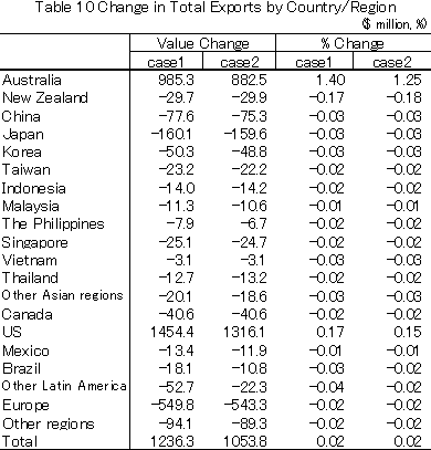
On the other hand, agricultural production decreases in the US because of the US-Australia FTA, and land prices decline. Table 9 as presented in the foregoing shows a decrease of 0.28% in Case 1 and 0.21% in Case 2. Meanwhile, the cost of labor and other production factors rise due to expansion in the non-agricultural sectors. However, growth is about 0.01%, except for natural resources. Generally the markets of production factors change less in the US than Australia. 4) Impact on Trade (i) By Country or Region Seeing the changes in total export by country or region in Table 10, the US's increase is greatest in monetary terms at $1,316.1 million in Case 2 but the percentage change is only 0.15%. On the other hand, Australia' increase amounts to $882.5 million, slightly lower than the US, but the percentage change is 1.25%, well above the US, and the greatest proportional change. Total global exports increase slightly by $1,053.8 million (+0.02%) but the total export changes in a negative direction everywhere except the US and Australia. New Zealand's decline is the sharpest, amounting to $29.9 million in Case 2 and at the rate of 0.18%. Japan's decrease amounts to $159.6 million, not small, but the percentage change is only 0.03%. Europe also decreases its exports largely by $543. 3 million in Case 2 but the percentage change is only about 0.02%.
(ii) Change in Exports from the US, Australia and Japan Table 11 shows the percentage change in export by destination from the US, Australia and Japan. Firstly Australia's exports to the US are expected to increase by 14.76% in Case 1 and by 10.61% in Case 2. And all its exports to countries other than the US decrease in Case 1 but increase in Case 2, except for those shipped to "other Asian regions". However, the percentage change in exports to third party countries is less than 0.5%. The percentage change in exports to Japan is only about 0.01% in Case 2.US exports to Australia increase by about 17% in both cases. US exports to third party countries decrease in both cases. US exports to Japan decrease by 0.16% in Case 2. Finally, the change in Japan's total exports by destination is examined; its exports to Australia decrease by 5.42% in Case 2 and to New Zealand drop by 0.30%. Its exports to other destinations all increase. Among them, exports to NAFTA countries increase comparatively widely. In Case 2 Japan's exports to Canada, the US and Mexico increase by 0.21%, 0.13% and 0.18% respectively. However, as already seen, Japan's total exports decrease and the increase in exports to NAFTA is far short of the decrease in exports to Australia and New Zealand.
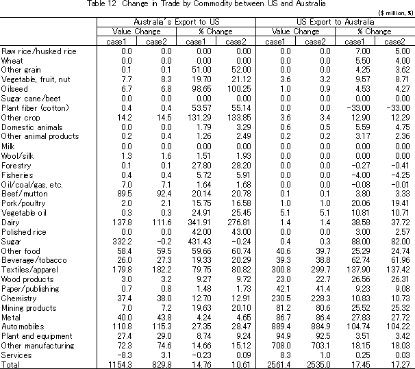
(iii) Change in Trade between the US and Australia Table 12 shows the change in the value of trade between the US and Australia by product. Among the products exported to the US from Australia, sugar shows a remarkably large change in Case 1. Sugar exports increase by $332.2 million or 431.43%. In Case 2, however, sugar exports decrease by $0.2 million (-0.24%). Meanwhile, the tariff barrier on dairy imports is largely reduced, and exports increase accordingly in either case. The increase is $137.8 million (+341.91%) in Case 1 and $111.6 million (+276.81%) even in Case 2. As tariffs are also lowered greatly on beef and mutton, exports increase by $89.5 million (+20.14%) in Case 1 and $92.4 million (+20.78%) in Case 2. Other than agricultural products, textile and apparel exports show a large increase; $299.7 million (+137.42%) in Case 2.
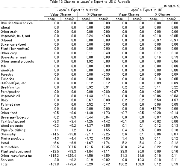
For the US's part, exports to Australia generally increase mainly for non-agricultural products. Car exports increase most by $884.9 million (+104.22%) in Case 2. Other manufacturing exports increase largely in dollar terms by $703.1 million but the percentage change is only 18.03%. Textile and apparel exports increase more than 100% by $299.7 million (+137.42%) in case 2. Turning to agricultural products, exports of vegetables, fruits and nuts increase by $3.2 million (+8.71%) in Case 2, and dairy exports by 1.4 million (+37.72%). Sugar exports show a large percentage change but the change in dollar terms is less than $1 million. (iv) Change in Japan- US Trade and Japan- Australia Trade According to Table 13, which shows a change in Japanese exports to the US and Australia by product, car exports to Australia decline most sharply both in dollar and percentage by $307.5 million (-12.35%) in Case 2. In other manufacturing industries, exports decrease significantly by $120.4 million (-4.59%). Meanwhile, car exports to the US slightly increase by $75.4 million (+0.23%), and other manufacturing industries also increase their exports by $34.0 million (+0.11%).
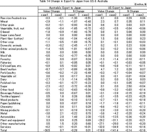
When the changes in export to Japan are inversely seen from the side of the US and Australia in Table 14, Australia's exports of many agricultural products decrease. Beef and mutton exports decrease by $3.7 million (-0.38%) and wheat exports are down by $1.1 million (-0.40%). Contrastingly, the US increases agricultural exports to Japan, mainly the same products for which Australia's exports decrease. Plant fiber (cotton) exports increase by $0.6 million (+0.23%) in Case 2, wheat by $0.7 million (+0.11%) and beef and mutton by $1.2 million (+0.07%) in Case 2. Because of the US-Australia FTA, weight shifts from Australia to the US for part of Japanese imports of agricultural products, but such shift is very minimal.
|
 248.5 billion, pork valued at